Multi-source data integration for soil mapping using deep learning

Wadoux, Alexandre M. J.-C.; Padarian, José; Minasny, Budiman

doi:https://doi.org/10.5194/soil-5-107-2019

Articles | Volume 5, issue 1

https://doi.org/10.5194/soil-5-107-2019

Articles | Volume 5, issue 1

Original research article

22 Mar 2019

Original research article |

| 22 Mar 2019

Multi-source data integration for soil mapping using deep learning

Alexandre M. J.-C. Wadoux, José Padarian, and Budiman Minasny

Abstract

With the advances of new proximal soil sensing technologies, soil properties can be inferred by a variety of sensors, each having its distinct level of accuracy. This measurement error affects subsequent modelling and therefore must be integrated when calibrating a spatial prediction model. This paper introduces a deep learning model for contextual digital soil mapping (DSM) using uncertain measurements of the soil property. The deep learning model, called the convolutional neural network (CNN), has the advantage that it uses as input a local representation of environmental covariates to leverage the spatial information contained in the vicinity of a location. Spatial non-linear relationships between measured soil properties and neighbouring covariate pixel values are found by optimizing an objective function, which can be weighted with respect to a measurement error of soil observations. In addition, a single model can be trained to predict a soil property at different soil depths. This method is tested in mapping top- and subsoil organic carbon using laboratory-analysed and spectroscopically inferred measurements. Results show that the CNN significantly increased prediction accuracy as indicated by the coefficient of determination and concordance correlation coefficient, when compared to a conventional DSM technique. Deeper soil layer prediction error decreased, while preserving the interrelation between soil property and depths. The tests conducted suggest that the CNN benefits from using local contextual information up to 260 to 360 m. We conclude that the CNN is a flexible, effective and promising model to predict soil properties at multiple depths while accounting for contextual covariate information and measurement error.

Download & links

Article (PDF, 5260 KB)

Download & links

How to cite

How to cite.

Dates

Received: 29 Oct 2018 – Discussion started: 16 Nov 2018 – Revised: 08 Feb 2019 – Accepted: 07 Mar 2019 – Published: 22 Mar 2019

1 Introduction

Digital soil mapping (DSM) techniques are commonly used to predict a soil property at unsampled locations using measurements at a finite number of spatial locations. Prediction is routinely done by exploiting the relationship between a soil property and one or several environmental covariates, which are assumed to represent soil forming factors. Examples of covariates are the digital elevation model (DEM) or its derivatives (Moore et al., 1993). Demattê et al. (2018) used multi-temporal and multispectral remote sensing images to map soil spectral reflectance while Nussbaum et al. (2018) investigated the use of a large set of covariates for mapping eight soil properties at four soil depths. The choice of covariates is governed either by their availability, preselected using a priori pedological expertise, or based on the pedological concepts whereby covariates must portray the factors of soil formation such as climate, organisms, relief, parent material and time (McBratney et al., 2018). In most cases, the relation between soil property and the chosen covariates is modelled by a regression model which relates either linearly (Wadoux et al., 2018) or non-linearly (Grimm et al., 2008) sampled (point) soil properties and a vector of covariate values extracted at the same point location.

Several authors have shown that this is not satisfactory (e.g. Moran and Bui, 2002). Pedogenesis and thus soil property spatial variation are governed by complex relationships with soil forming factors and landscape characteristics, materialized at a local, regional or supra-regional scale (Behrens et al., 2014). Point information of the covariates can only describe approximately the soil property because a large part of the spatial contextual information is missing. For example, soils on a gentle slope might have a great accumulation of soil organic matter, accumulation which varies according to the surrounding slope gradients. Several studies have shown that incorporating covariate contextual information improves prediction accuracy (Behrens et al., 2014; Grinand et al., 2008; Gallant and Dowling, 2003). Smith et al. (2006) tested different neighbouring size in computing terrain attributes for use in a soil survey. The authors showed that the amount of contextual information supplied to the model significantly impacts the output of the survey. In spite of these conclusions, contextual information surrounding a sampling location is usually disregarded in DSM studies.

Several attempts have been made to incorporate the spatial domain of the covariates into the analysis. Behrens et al. (2010 a) developed ConMAP, which computes the elevation difference from the centre pixel to each pixel in a neighbourhood, and ConStat (Behrens et al., 2014), which derives statistical measures of elevation within a growing radius of the centre pixel. This generates a very large number of hyper-covariates, abstract representation of the context, which can be used as predictors in subsequent regression models. Another approach uses spatial transformations such as wavelet transform to represent the covariate as a function of various local spatial supports (e.g. Lark and Webster, 2001). Alternatively, one may account for contextual information by simply using covariates aggregated at larger support than their original resolution (Miller et al., 2015). This technique, referred to as the multi-scale approach, provides a surprisingly large increase in prediction accuracy. It is now acknowledged that using covariates with coarse spatial resolution can provide satisfactory prediction (Samuel-Rosa et al., 2015).

However, while these approaches enable us to contextualize the spatial information supplied to the regression, they rely either on heavy covariate preprocessing (Behrens et al., 2014), subjective decisions based on the resolution to which covariates must be treated as input to the model (Miller et al., 2015) or the modeller's choice regarding neighbouring size (Behrens et al., 2010 b). In light of these drawbacks, we propose the use of the convolutional neural network (CNN) as an alternative tool for mapping while explicitly accounting for local contextual information contained in covariates. Recently, Padarian et al. (2019) have shown that it is possible to use the CNN for soil mapping while accounting for contextual covariate information, whereas Behrens et al. (2018) compared the deep neural network to the random forest model for mapping and found that the former model provides more accurate predictions. In Behrens et al. (2018), the covariates must still be preprocessed. The authors used a deep learning architecture which uses a vector as input. The CNN proposed here has the advantage that it relies on the local representation of covariates so as to leverage the spatial information contained in the vicinity of a sampled point. The CNN uses an image as input, does not require any preprocessing of the input covariates and performs a multi-scaling analysis directly on the image (Padarian et al., 2019). As for other regression methods, the CNN is trained using measured soil properties at the point location.

Measured soil properties are never error-free. Soil measurements can be best performed under controlled conditions in the laboratory. In the latter case, the error of those measurements is small and their impact on prediction is safely ignored. With the advent of new technology, soil measurements are often inferred using sensors such as spectrometers. The result is the creation of databases of soil properties measured or inferred using several sensors which predicted soil properties with different accuracy levels. Recently, Ramirez-Lopez et al. (2019) and Somarathna et al. (2018) have shown that measurement error may have a significant impact in subsequent spatial analysis. For example, Ramirez-Lopez et al. (2019) estimated a measurement error of about 50 % for top- and subsoil ${Ca}^{+ +}$ inferred using near-infrared (NIR) spectroscopy. In most cases, measurement error can be quantified and must therefore be accounted for when calibrating a spatial model using uncertain measurements. While Padarian et al. (2019) demonstrated the use of the CNN for mapping at a country scale, we further advanced this concept for mapping soil properties at a landscape scale, which considers the measurement error of soil measurements.

The objectives of this study are to (i) develop the framework of the convolutional neural network for contextual spatial modelling at a regional scale, (ii) develop a methodology for multi-source data integration by accounting for the soil property measurement error in the CNN model calibration, and (iii) demonstrate the usefulness of the CNN to map top- and subsoil organic carbon in a potential application scenario.

2 Methodology

2.1 Artificial neural network

We first describe the principle of an artificial neural network (ANN), which is the basis of the CNN. A measured soil property of interest $z_{s_{i}}$ at location $s_{i} (i = 1, \dots, n; s_{i} \in A)$ in the study area 𝒜 is modelled by a regression model:

\begin{matrix} (1) & z_{s_{i}} = f (X_{s_{i}}; θ) + ε_{s_{i}}, \end{matrix}

where X is either a $c \times (w \times h)$ 2-D matrix or a 3-D input matrix of size $c \times w \times h$ which contains c environmental covariates of size w×h pixels centred at spatial location s_i. The vector θ represents model parameters used by the neural network regression model f to map non-linearly X→z and leave room for a zero mean random error ε. Note that, unlike geostatistics, measurements of the soil property are assumed to be spatially independent and identically distributed.

An ANN model is formed of several layers, or “computation steps”. The input layer provides the raw information to the network (see h⁰ in Fig. 1b), which is connected to at least one hidden layer (h^k in Fig. 1b), which in turn is connected to an output layer (h^L in Fig. 1b), which outputs the predictions of interest $z_{s_{i}}$ . Each layer contains units called nodes for the input layer (as no computation occurs at their level) and neurons for the hidden and output layers (Fig. 1a). The behaviour of the neurons depends on the activity of the previous layer neurons and the connection weights between the previous and next layer neurons (LeCun et al., 2015). The parameters of the models defined by Eq. (1) are thus the connection weights to the neuron j, $w_{j} = (w_{j, 1}, \dots, w_{j, l})$ , and a bias component per neuron b_j. They are associated with an activation function ϕ which gives output z_j by

\begin{matrix} (2) & z_{j} = ϕ (〈 w_{j}, x 〉 + b_{j}), \end{matrix}

where $〈 \cdot, \cdot 〉$ is the dot product and x is a vector of inputs from previous layer neuron output. A graphical representation is provided in Fig. 1a. In this study we use the rectified linear unit (ReLU) activation function $ϕ (x) = \max (0, x)$ while the output layer for regression uses the linear activation function $ϕ^{'} (x) = x$ . Equation (2) shows that the activation function determines the output of a neuron by applying a linear or non-linear transform on the input.

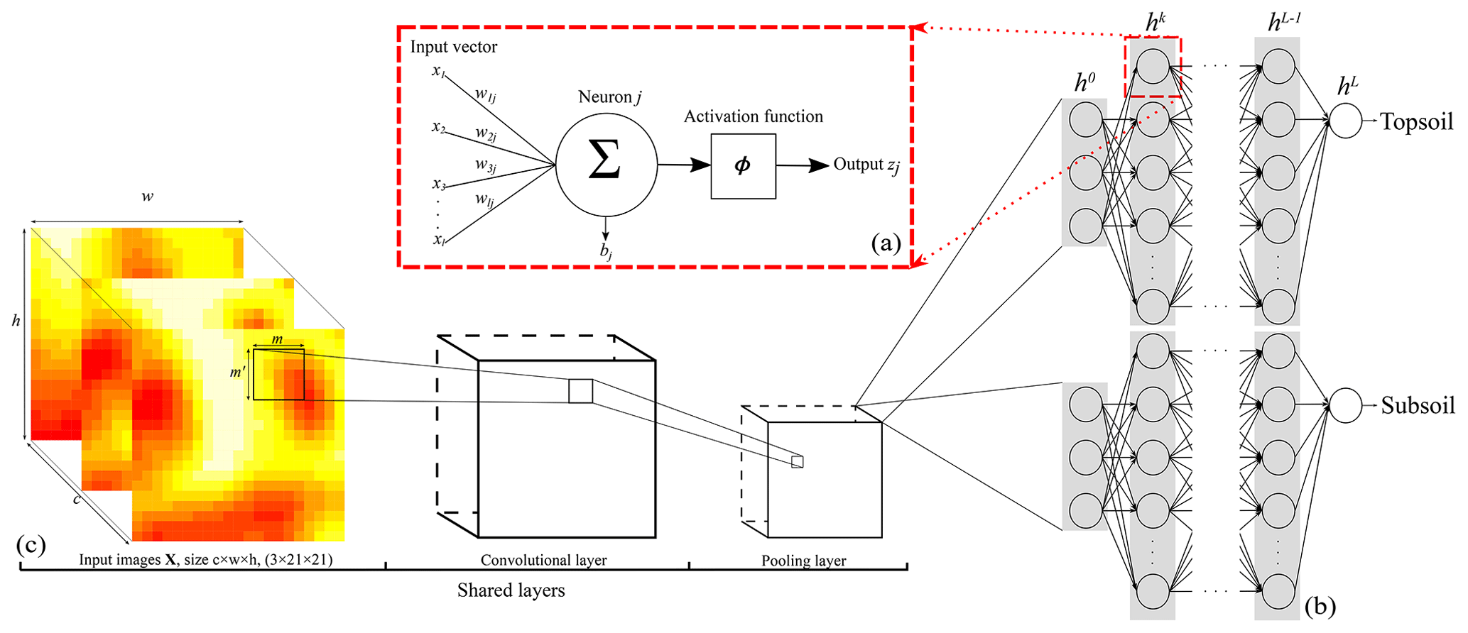
https://www.soil-journal.net/5/107/2019/soil-5-107-2019-f01

Figure 1Representation of the CNN architecture developed in this study for (a) a neuron, (b) the ANN architecture or fully connected layer, and (c) the convolutional and pooling layers. Note that $\sum = 〈 w_{j}, x 〉$ . The size of the output from a convolutional or pooling layer (c) is smaller than that of its input. Panel (c) is the shared structure to extract common features between the two depths which is then separated into two branches (one per soil depth) in (b).

Download

Our neural network will contain more than one single hidden layer. For $k = 1, \dots, L$ hidden layers h and an input layer h⁰ where no processing occurs (Fig. 1b):

\begin{array}{l} (3) & h^{0} (x) & = x, \\ (4) & h^{k} & = ReLU (W^{k} h^{k - 1} (x)), for k = 1, \dots, L - 1, \\ (5) & h^{L} & = W^{L} h^{L - 1} (x) . \end{array}

For each layer, W is a matrix of size $J^{k} \times J^{k - 1}$ , i.e. the number of neurons in the current layer by the number of neurons in the previous layer. Therefore the model parameters $θ = (W^{1}, b^{1}, \dots, W^{L}, b^{L})$ .

2.2 Convolutional neural network

In this paper we use the vicinity information of the measured soil property by including the covariate pixel values surrounding a sampling location. In this case, an ANN is not well adapted because it uses vectors as input data, while (correlated) spatial information is better represented as images. In the convolutional neural network, at least one layer is a convolution (Goodfellow et al., 2016), i.e. an element-wise product and sum between two matrices. Let there be an input image matrix X, e.g. a digital elevation model cropped for size w×h pixels surrounding a measured soil property at location s_i. We apply a 2-D convolution using the filter F of size m pixels × m^′ pixels to the input image X such that

\begin{matrix} (6) & (F * X)_{(w, h)} = \sum_{m, m^{'}} F_{(m, m^{'})} X_{(w + m^{'}, h + m)}, \end{matrix}

which can be rewritten with little modification to include the case where we have c=3 environmental covariates (Goodfellow et al., 2016, Eq. 9.4). Equation (6) shows that each element in (F∗X) is calculated as the sum of the products of one element in X and one element in F. In other words, the elements of (F∗X) are the sum of the element-wise multiplication of F by X. The size of the output image from a convolution is thus smaller than that of its input image (see Fig. 1c).

Filters detect features (e.g. edges) related in the vicinity of a sampling location and leverage the spatial structure of the covariates. In practice, the original covariate image goes through several filters, each exploiting an abstract representation of the image features. Similar to the ANN, the CNN has a number of hidden layers, called convolutional layers. The convolutions are combined with an activation function at the end of each neuron, obtained by

\begin{matrix} (7) & z_{j} (X) = ϕ (F^{L} * h^{L - 1} + b_{j}) . \end{matrix}

In addition to the convolutional layers, another set of operations consists of pooling layers. Pooling reduce the spatial size of the images by down-sampling along the spatial dimension. Several types of pooling operations exist, such as minimum, maximum or average pooling. The most common is the max-pooling operation, which consists in selecting the maximum value in the convoluted image using a given filter size. Each convolution accepts one input image of a given size and number of channels, i.e. covariates, and returns another image of possibly a different size and number of channels. Usually, one wants to reduce the size of each image at each convolution while augmenting the number of channels. Then, the last convolution returns an image of size 1×1 and with a number of channels. This operation is named “flattening”, as it converts the matrices into a vector which can pass to a fully connected layer. A fully connected layer is an ANN layer, as noted in Fig. 1b. The large number of connections between neurons generates a high number of parameters which can provoke overfitting. This can be restrained by introducing dropout layers which randomly disconnect a number of neurons. Usually, the dropout rate is no greater than 0.5.

2.3 Parameter estimation

The CNN model is trained on dataset $D = {(X_{s_{i}}, z_{s_{i}}) \dots (X_{s_{n}}, z_{s_{n}})}$ , that is, a 4-D matrix of size $n \times c \times w \times h$ . The dataset 𝒟 is used to derive an optimized value of the parameters $\hat{θ}$ for θ by minimizing the mean squared error (MSE) as the objective function, given by

\begin{matrix} (8) & MSE = \frac{1}{n} \sum_{i = 1}^{n} δ_{i} (z_{s_{i}} - \hat{f} (X_{s_{i}}; \hat{θ}))^{2}, \end{matrix}

where δ are the measurement error weights, which are all 1 if the soil property is measured without error. In this study, we used the Adam optimizer (Kingma and Ba, 2015) to minimize Eq. (8). The Adam optimizer uses the derivative of the objective function with respect to each model parameter to update its value. This process is called backpropagation (LeCun et al., 1989). The optimization process runs for a number of epochs. An epoch describes the number of times the network sees the entire input dataset. During each epoch, the entire dataset is shown to the network in small subsets shuffled at random, called “minibatches”. The number of epochs must be chosen, as well as the batch size. In addition, one must choose the learning rate of the optimizer, i.e. how fast the optimizer moves the connection weights in the opposite direction of the gradient after each update. A too-small learning rate increases the computation time to find the optimum of the objective function because the steps are small. If the learning rate is too large, training may not converge because the connection weights oscillate. The learning rate can be tuned as other model architecture hyperparameters. This is explained in the next sections.

2.4 Multi-source data integration

The values of the soil property $z_{s_{i}}$ used to train the CNN model might be uncertain. For example, they are derived using an infrared spectroscopy model. This uncertainty must be accounted for when calibrating the CNN model. A solution is to assign a measurement error weight to each value of the soil property, depending of its relative error compared to a “true” measurement of the soil property at the same location. We refer to the “true” measurement of a soil property as a measurement made using a standard laboratory technique which has a small error. Meanwhile the spectroscopically inferred property is the value predicted using measurements from an infrared spectrometer. The prediction is based on a calibration model that relates observations of spectra and their true measurement values. For a vector of a soil property inferred using a spectroscopic model z_IR, one can assign a measurement error weight by comparing the variance of the predicted soil property by the infrared model to the variance of the measurements used for the infrared model calibration. The measurement error weight δ is given by

\begin{matrix} (9) & δ = 1 - \frac{var (z_{IR})}{var (z)}, \end{matrix}

which can then be applied to weight the importance of the values of the soil property inferred by the infrared model, at locations where the true soil property is unknown. Note that while all measurements have a measurement error weight, the same value of measurement error is used for a given spectroscopic model (NIR or MIR) and soil depth. In this work, a true value of a soil property is measured in the laboratory, with assigned measurement error weight of 1. The measurement error weights for each observation are used in model calibration, by updating the objective function to minimize in Eq. (8).

2.5 Quality of predictions

Once model parameter vector θ values have been estimated, they are used to predict at a new, unobserved location s₀ by

\begin{matrix} (10) & {\hat{z}}_{s_{0}} = \hat{f} (X_{s_{0}}; \hat{θ}), \end{matrix}

which is used to evaluate the prediction accuracy on an independent test set. Let there be N−n independent test locations $s_{i}, i = (N - n), \dots, N)$ where N is the total number of measurements and n is the set of samples used for calibration, generally 80 % of the measured values. We quantify the quality of predictions by the root mean squared error (RMSE) and the R². The bias is assessed by the mean error (ME),

\begin{matrix} (11) & ME = \frac{\sum_{i = 1}^{N - n} (z_{s_{i}} - {\hat{z}}_{s_{i}})}{N - n}, \end{matrix}

and the agreement of the predictions to the measurements with respect to the 1:1 line is assessed by the concordance correlation coefficient (ρ) (Lawrence and Lin, 1989):

\begin{matrix} (12) & ρ = \frac{2 ρ^{'} σ_{z} σ_{\hat{z}}}{σ_{z}^{2} + σ_{\hat{z}}^{2} + (μ_{z} - μ_{\hat{z}})^{2}}, \end{matrix}

where μ and σ² are mean and variance for either the vector of true measurements z or the vector of predicted values $\hat{z}$ . The value ρ^′ represents the correlation between μ_z and $μ_{\hat{z}}$ .

3 Case study

3.1 Study area and data

We tested the methodology in a 220 km² area located in the lower Hunter valley area, Australia. Elevation ranges from 27 to 322 m above sea level with a pronounced slope ascending in the south-west direction. Measurements of the total soil carbon (TC) expressed in g 100 g⁻¹ are available for topsoil (0–10 cm) and subsoil (40–50 cm). There was inorganic carbon in the measurements of the TC. Especially in the second depth, some of the large TC values are due to inorganic carbon. The lower Hunter area measurements were surveyed along several years, which yielded the use of three TC measurement methods, referred to as CNS, NIR and MIR hereafter.

Laboratory analysis (CNS). Soil samples were analysed for TC using the dry combustion method, i.e. by determining the loss on ignition at 400 ^∘C under controlled conditions. This was done by an Elementar Vario Max CNS analyser (Elementar Analysensysteme GmbH, Hanau, Germany). The standard deviation of the TC values inferred by the latter device is small (less than 0.004 g 100 g⁻¹).
Inferred using near-infrared (NIR) spectroscopy. Soil samples were scanned in the NIR range using an AgriSpec portable spectrophotometer with a contact probe attachment (Analytical Spectral Devices, Boulder, Colorado). TC values were inferred using a spectroscopic model calibrated by the cubist regression tree method, using the spectral library of 316 soil samples from Geeves et al. (1995).
Inferred using mid-infrared (MIR) spectroscopy. Soil samples were scanned in the MIR region using a Bruker Tensor 37 Fourier transform spectrometer. TC values were inferred using the MIR calibration model defined by Minasny et al. (2008).

A large number of locations contain more than one single measurement of TC. This is particularly visible in the western part of the area, where many samples have been analysed using the two or three methods, and with a replication (Fig. 2). In total, 2388 measurements of TC are available for the first depth, among which 645 are from the CNS methods, 923 are from the NIR method and 820 are from the MIR method. In the second depth, there are 2058 measurements of the TC: 187 using the CNS method, 999 using the NIR method and 872 using the MIR method. They are shown in Fig. 2.

In addition to the TC measurements, three covariates from the study of Somarathna et al. (2018) at 25 m×25 m resolution were used:

A digital elevation model from the SRTM (Shuttle Radar Topography Mission) (Fig. 3a); see Farr et al. (2007).
A map of the Landsat 5 ETM band 5 (Fig. 3b), which corresponds to the shortwave infrared (SWIR) band for the wavelength 1.55–1.75 µm.
A map of the normalized difference vegetation index (NDVI) (Fig. 3c), derived from the NIR (band 4) and red (band 3) of the Landsat 5 ETM sensor.

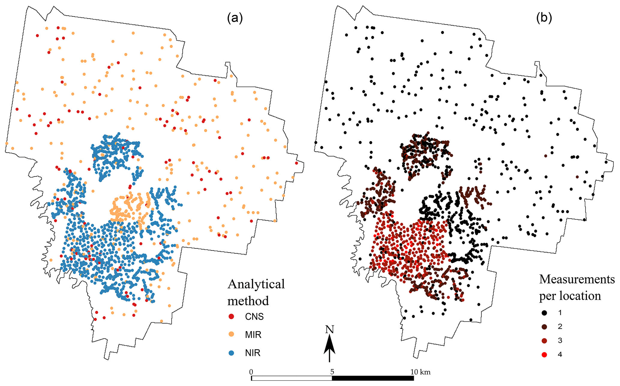
https://www.soil-journal.net/5/107/2019/soil-5-107-2019-f02

Figure 2Spatial distribution of the observations for each measurement type (a) for the 0–10 cm topsoil and (b) number of measurements recorded per sampling location for the 0–10 cm topsoil. The subsoil (40–50 cm) map is not shown but closely resembles the topsoil in both number of sampling locations and number of measurements per location.

Download

https://www.soil-journal.net/5/107/2019/soil-5-107-2019-f03

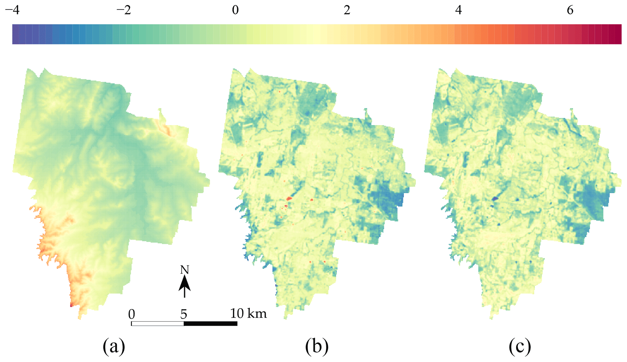
Figure 3Standardized covariates used in model calibration (a) DEM, (b) Landsat 5 ETM band 5 and (c) NDVI.

Download

3.2 Practical implementation

3.2.1 Model definition

The dataset of TC measurements was randomly split between test (20 %) and calibration (80 %) sets. Both topsoil and subsoil measurements were jointly selected for either test or calibration. All soil measurements were normalized between 0 and 1 using the minimum and maximum values of the calibration set. In addition, all covariates were centred on 0 and scaled to a standard deviation of 1 (see Fig. 3). Next, two 4-D matrices of dimension $n \times c \times w \times h$ and $(N - n) \times c \times w \times h$ were created (test and calibration), where n is the number of calibration TC measurements, N−n is the number of test measurements, c is the number of covariates and w=h is the vicinity size (the square matrix) surrounding the TC measurements. We have n=3557 for calibration and $(N - n) = 889$ for test, as well as c=3 and w=h of different sizes. When a square of size w×h is created in the vicinity of a soil property at the border of the area, several missing values are reported. Since the CNN can not handle this type of input, we assigned to the missing values the number −1. This practical problem is discussed more extensively in the Discussion section.

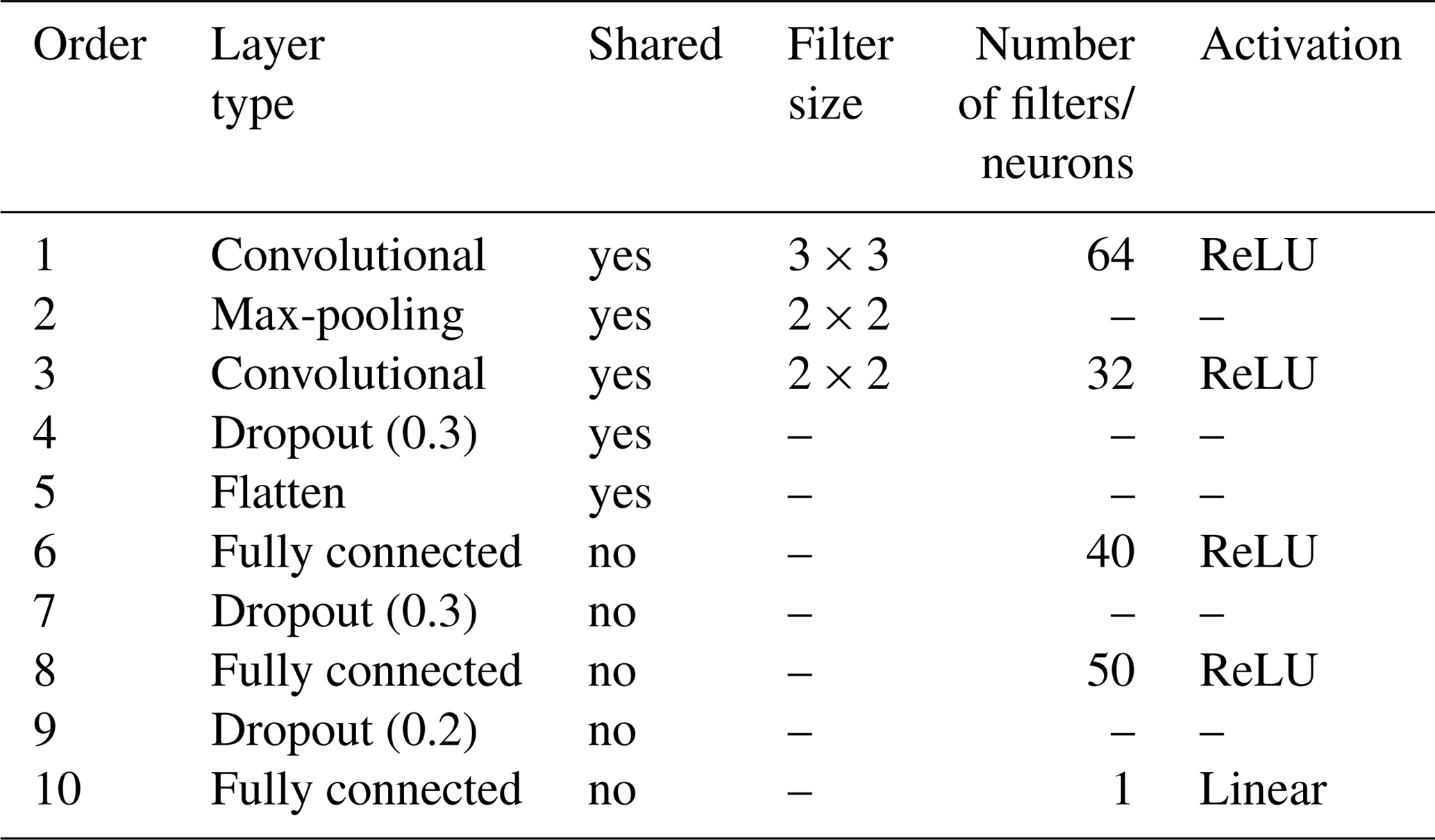
A sequential multitask (top- and subsoil) CNN model was built. The CNN is composed of a common architecture for the two soil depths (shared layers) followed by two separate sets of fully connected layers, one for each soil depth. An illustration of the model is provided in Fig. 1b–c. The model specifications are reported in Table 1. Note that for the convolutional layers, zero padding is always applied to the original input image before the dot product with the filters. This operation keeps the original size of the input image and preserves its information at an early stage of the model. We use the max-pooling operator; i.e. we select the maximum value in the convoluted image using a given filter size, in our case a filter of size 2 pixels × 2 pixels.

Table 1Layers used in the sequential model built for topsoil and subsoil TC prediction.

Download Print Version | Download XLSX

In order to compare the CNN prediction to a reference method, we also calibrated two random forest (RF) models, one per soil depth. Random forest is a non-linear machine learning method which has been widely used for soil mapping. For more information, the reader is redirected to Hengl et al. (2018). For a fair comparison between the CNN and RF models, we used the same calibration and test sets, with normalized TC measurements and standardized covariates as input. A RF model is calibrated for each soil depth, using depth-specific fine-tuned parameter values.

3.2.2 Parameter estimation

Once the sequential CNN model was specified, the parameters were estimated by minimizing the MSE as the objective function (Eq. 8), for which we used the Adam optimizer. Overfitting was carefully checked by (i) modifying the dropout rate in the model and (ii) ensuring that the model does not provide a considerably larger objective function on an independent dataset. Since the test set was used solely to validate the predictions, it could not be used for this purpose. We therefore randomly split the calibration set into two sets, referred to as the calibration and validation sets hereafter. The calibration set (90 %, 3201 measurements) was used to calibrate the model, and the validation set (10 %, 356 measurements) was used to tune the parameters and prevent overfitting.

The model was trained using different window sizes of the input images. We compared a model with a window size (w×h) of 3, 5, 9, 15, 21, 29 and 35 covariate pixels for the input. The comparisons were made based on the average between the two depths' RMSE of the predictions, made on the validation set. Optimization of the parameter of a single model (Table 1) using three covariates, an input window size of 21×21 and 3557 TC measurements took approximately 1 h in parallel on a standard four-core laptop. All processing was done in R 3.5.1 (R Core Team, 2018), using the keras package (Allaire and Chollet, 2018) and tensorflow (Abadi et al., 2016) backend.

Once the input window size was selected, the hyperparameters of the model architecture were optimized using Bayesian optimization (Snoek et al., 2012). Note that this is different from the optimization of the objective function using the Adam optimizer. In Bayesian optimization, the objective function is treated as a random function characterized by a prior probability distribution. Each function evaluation is treated as data, which enables updating the objective function posterior distribution. The latter is used to determine where to evaluate next. The process is repeated until reaching a stopping criteria. Bayesian optimization enables us to find optimized values of machine learning hyperparameters with commonly less iteration than when using a random search. In this work, we optimized the filter number, the neuron number, the batch size and the learning rate using 50 iterations.

4 Results

Based on the procedure detailed in Sect. 2.4, measurements of TC inferred from NIR spectra were assigned a measurement error weight of 0.43 and 0.52 for topsoil and subsoil, respectively. The MIR-inferred TC measurements had a measurement error weight of 0.62 for topsoil and 0.61 for subsoil. This suggests that the MIR range of the spectra is more accurate in predicting TC. Recall that all CNS-inferred measurements had a measurement error weight of 1, as explained in the previous section.

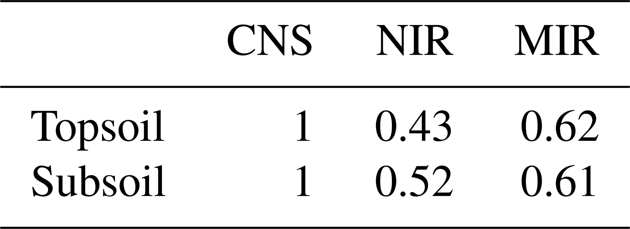
Table 2Weights given to the measurements.

Download Print Version | Download XLSX

Figure 4 shows the RMSE of topsoil and subsoil TC for different vicinity size of the input images. Contextual information is accounted for by representing the input data as images of a square format surrounding a soil measurement. Each pixel has a resolution of 25 m×25 m so that a window of size 3×3 includes contextual information up to $3 / 2 \times 25 = 37.5$ m. For both soil depths, Fig. 4 shows a similar pattern with increasing size of the window. The RMSE becomes significantly smaller when using a larger window of size 5×5. The lowest averaged (topsoil and subsoil) RMSE is found for a window size of 21×21 (radius of about 262 m). It seems that model calibration does not benefit from using a larger window size as the RMSE increases for a window size of 29×29 and 35×35. From now on, all the results presented come from using an input window size of 21 pixels × 21 pixels.

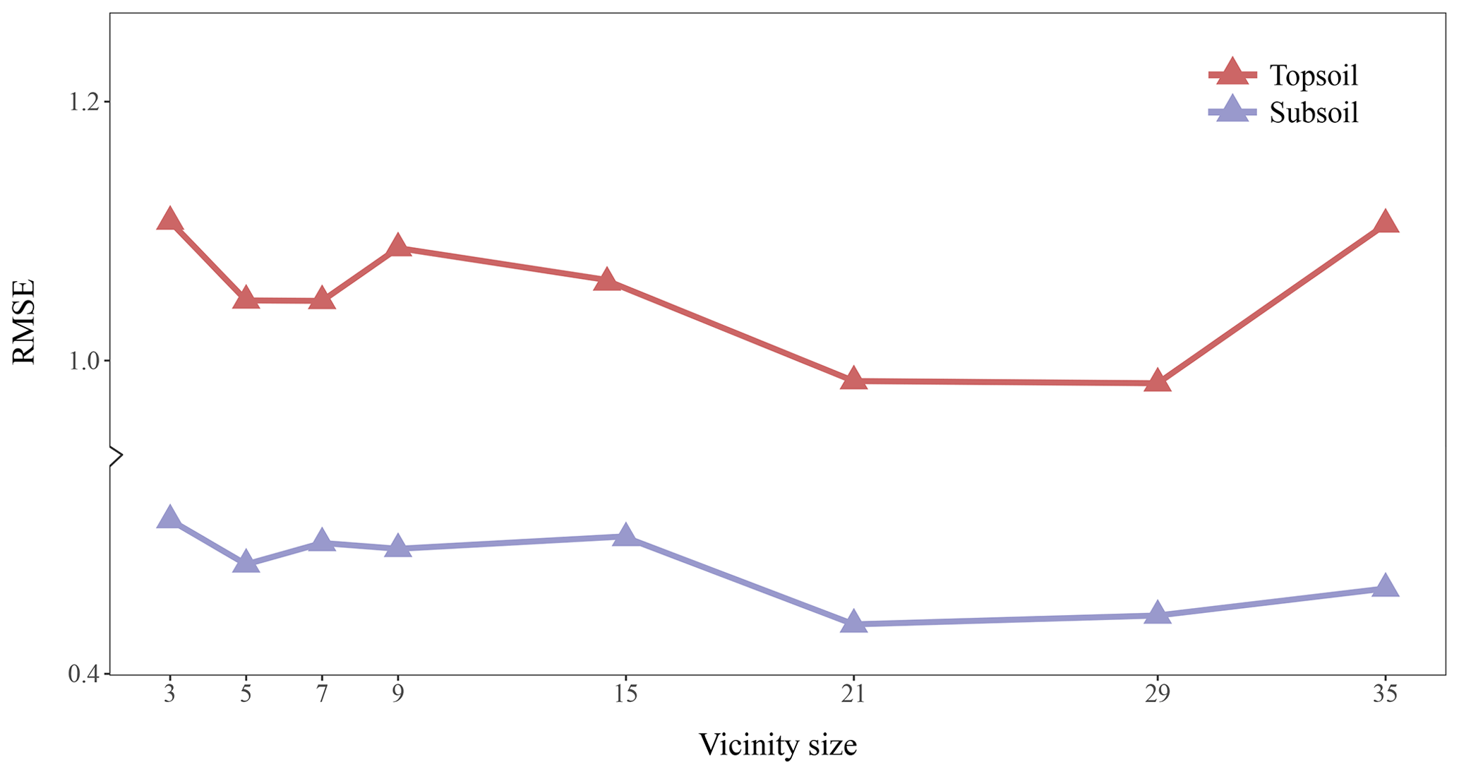
https://www.soil-journal.net/5/107/2019/soil-5-107-2019-f04

Figure 4Effect of the vicinity size of input images. The RMSE (in g 100 g⁻¹) corresponds to the error between the predictions and measured values in the test set.

Download

The scatterplots of the measured against predicted TC values are presented in Fig. 5 for both the CNN and RF models. For the CNN model, the agreement between measured and predicted TC was found to be satisfactory for both soil depths. Topsoil predicted TC tends to be underestimated for large measured values of TC. This is also the case for subsoil where large measured values of TC (e.g. 7.5 and 8 g 100 g⁻¹) have smaller predicted values at around 4 g 100 g⁻¹. There is a high density of predicted values close to the 1:1 line. In contrast to the CNN model, the predictions using the RF model are more dispersed, with several over-predicted values for the low range of the measured TC values. Visual inspection of Fig. 5 suggests that the CNN model predicts more accurately than the RF model.

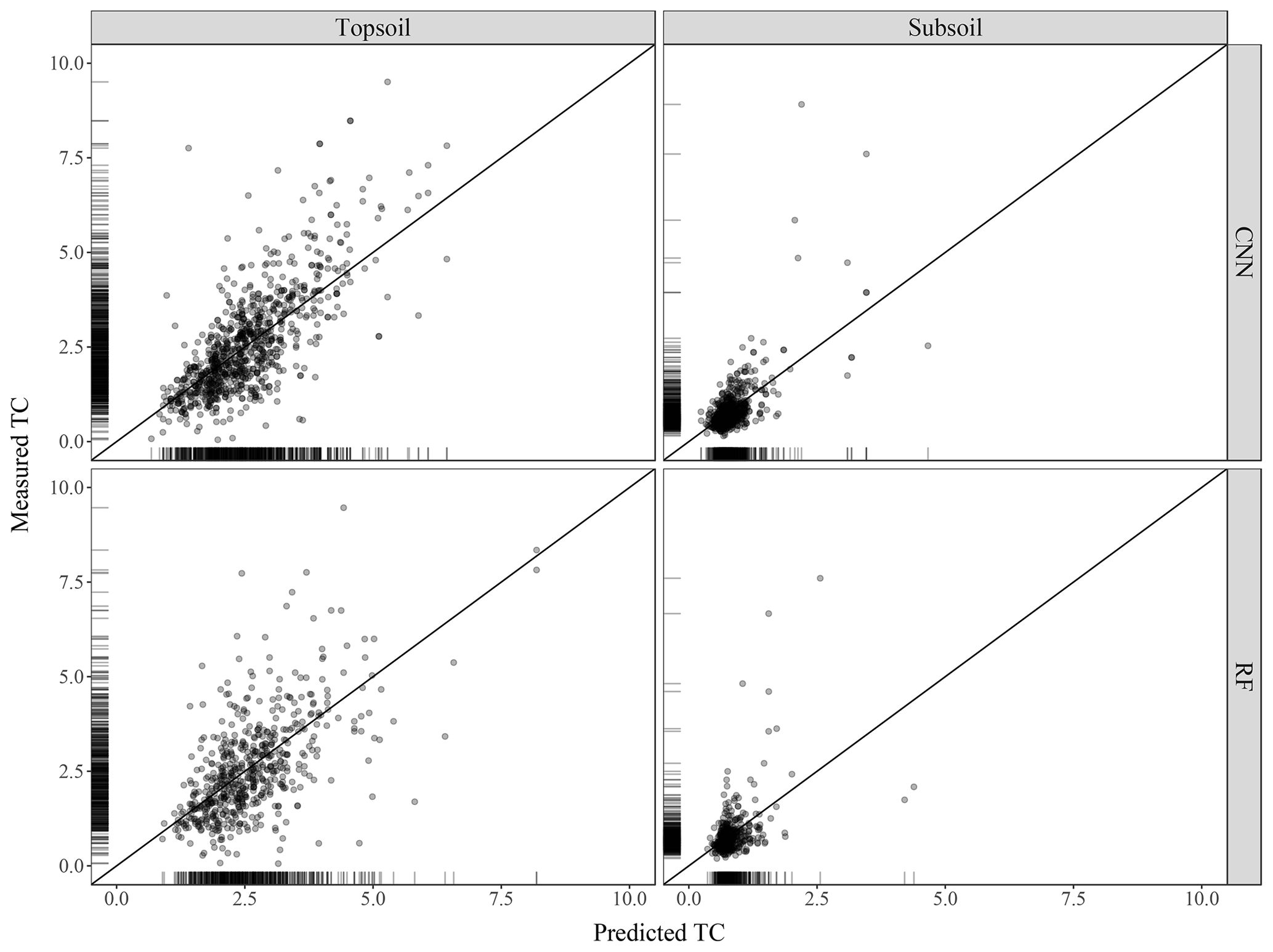
https://www.soil-journal.net/5/107/2019/soil-5-107-2019-f05

Figure 5Scatterplot of the measured against predicted topsoil and subsoil TC for the CNN and RF models, along with the 1:1 line. Values are expressed in g 100 g⁻¹.

Download

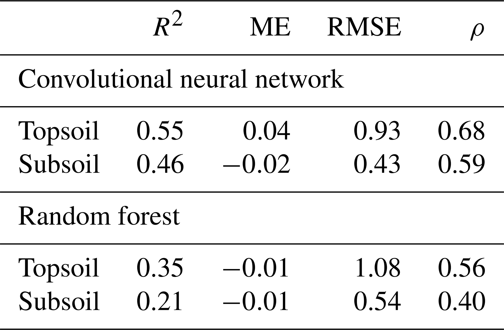
This is confirmed by the quantitative assessments of the predictions shown in Table 3. Correlation between predicted and measured TC, as measured by the R², is stronger for the CNN (R²=0.55 for topsoil and R²=0.46 for subsoil) than for the RF model (R²=0.35 for topsoil and R²=0.21 for subsoil). The ME (in g 100 g⁻¹) shows that predictions for both models are relatively unbiased (ME close to zero in all cases). The CNN model provides a significantly smaller accuracy measure (topsoil RMSE of 0.93 against 1.08 for the RF model) while providing as well a larger degree of prediction falling on the 45^∘ line through the origin (about 15 % higher for both topsoil and subsoil), as already noticed visually in Fig. 5.

Table 3Evaluation of prediction accuracy on the independent test set (R² – coefficient of determination; ME – mean error, in g 100 g⁻¹; RMSE – root mean square error, in g 100 g⁻¹; ρ – Lin's concordance coefficient).

Download Print Version | Download XLSX

The maps produced using the CNN are shown in Fig. 6 for topsoil (left) and subsoil (right) soil organic carbon. Both maps have a relatively smooth pattern. The topsoil map of TC shows the highest concentrations in the south-east border of the area (>8 g 100 g⁻¹), with a relatively large concentration in the centre of the area (5 g 100 g⁻¹). There seems to be more TC in areas where the NDVI has large values, but this pattern is not obvious. The subsoil maps of TC have a very different pattern than the topsoil map. There seems to be a uniform distribution of TC around 1 g 100 g⁻¹ for most of the area. High concentrations of TC (>5 g 100 g⁻¹) are seen in a patch in the centre of the catchment and in a large area in the south.

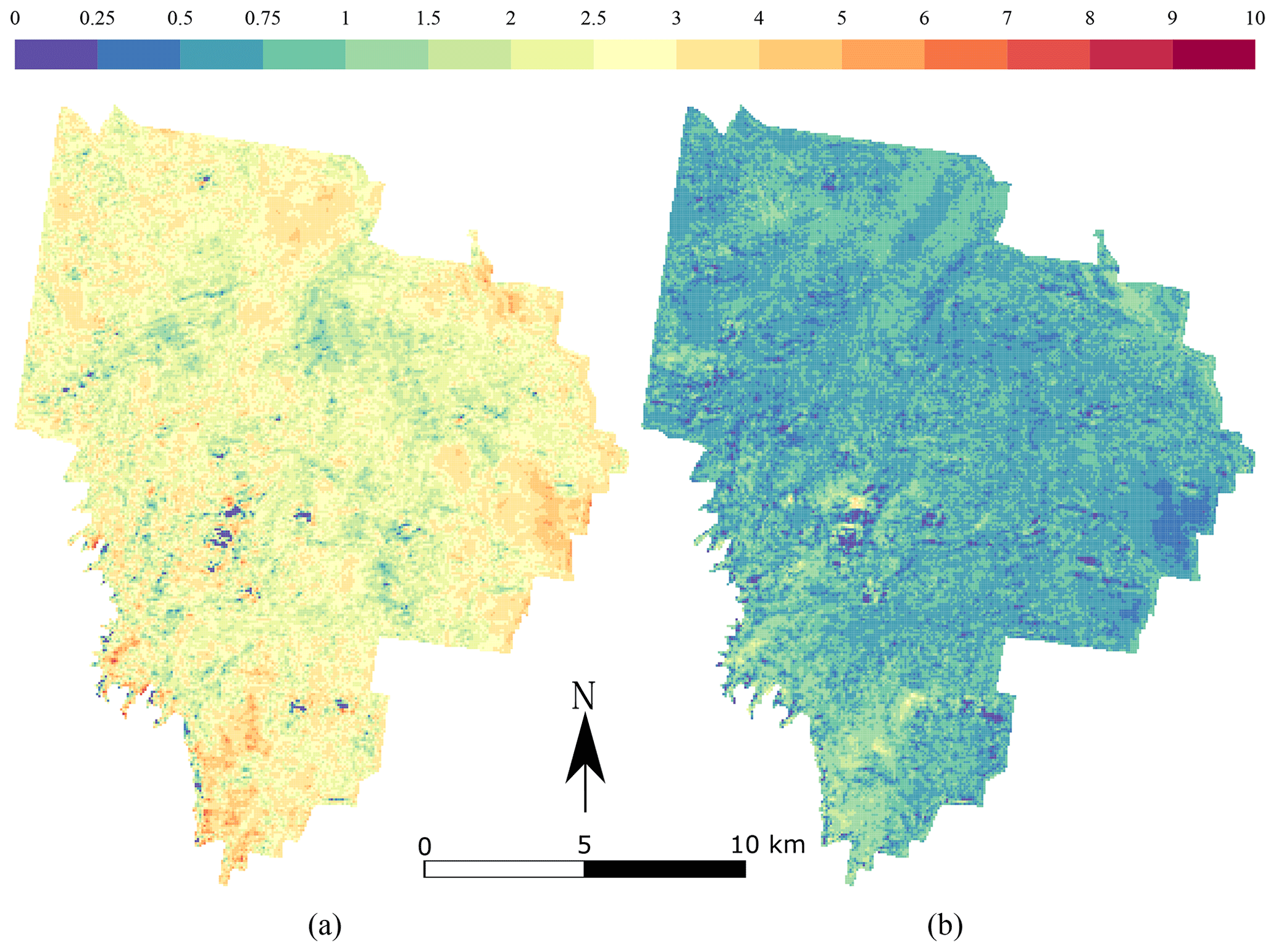
https://www.soil-journal.net/5/107/2019/soil-5-107-2019-f06

Figure 6Maps of the prediction of organic carbon for (a) topsoil (0–10 cm) and (b) subsoil (40–50 cm). The values are expressed in g 100 g⁻¹.

Download

5 Discussion

The proposed modelling approach explicitly accounts for the TC measurement error in the model calibration. The measurement error of NIR-inferred TC was larger than that of the MIR-inferred TC. This is an expected result reported in many previous studies (e.g. Rossel et al., 2006). The reason is that fundamental molecular vibration of bands associated with soil organic constituents occurs in the MIR region, while overtones and combinations appear in the NIR. Accounting for measurement error in spatial modelling of soil property using spectroscopically inferred soil data received recently much attention. Using the same case study, Somarathna et al. (2018) showed that acknowledging for measurement error almost halved prediction uncertainty. Similarly, Ramirez-Lopez et al. (2019) emphasized the importance of estimating and accounting for measurement error of spectroscopically inferred soil properties, as those can be larger than the sampling error. To the best of our knowledge, our study is one of the first to account for measurement error for mapping using machine learning. We note the contribution of Hengl et al. (2018), who used the measurement error to change the probability of a measurement to be selected in the bootstrap sample to calibrate a RF model.

The window size of the input images had a significant impact on the model's accuracy measure, as tested on an independent test set. This is because the size of the input image is closely related to the amount of contextual information we supply to our model. The CNN integrates spatial context by using the pixels of covariates surrounding a sampling location. In our regional-scale case study of TC mapping, a window size of 21 pixels × 21 pixels and 29 pixels × 29 pixels provided the lowest prediction error, but larger window size worsened the prediction accuracy. In a similar context, this confirms the results found by Behrens et al. (2010 b). The authors showed that prediction accuracy of topsoil silt content increased remarkably by using larger neighbourhood size. However, our results also clearly indicated that including larger-scale contextual information (larger input image window size) is not always better. This is similar to the results of Smith et al. (2006), who noted that the windows size greatly varies between landscapes and concluded that the appropriate size is case-dependent.

Using a window size of 21 pixels × 21 pixels and 29 pixels × 29 pixels is equivalent to including spatial information in a radius from the sampling location of about 262 to 362 m. Thus, it can be assumed that the window size relates to the range of spatial autocorrelation of TC. Several authors provided equivalent values of the spatial correlation range. Kumhálová et al. (2011) reported values of the organic matter spatial correlation range between 240 and 270 m using data of an experimental field in the Czech Republic. Similarly, Jian-Bing et al. (2006) found a spatial correlation range of 309 m for a small watershed in northeast China. For our case study, we verified this assumption by fitting a spherical variogram to the experimental variogram of TC. The fitted value of the range was 329 m for the topsoil and 275 m for the subsoil. This is close to the actual radius of the window size that we found optimal. It is however difficult to draw conclusions based on the results. The actual correlation between the autocorrelation range of a soil property and window size deserves further investigation so as to generate rules.

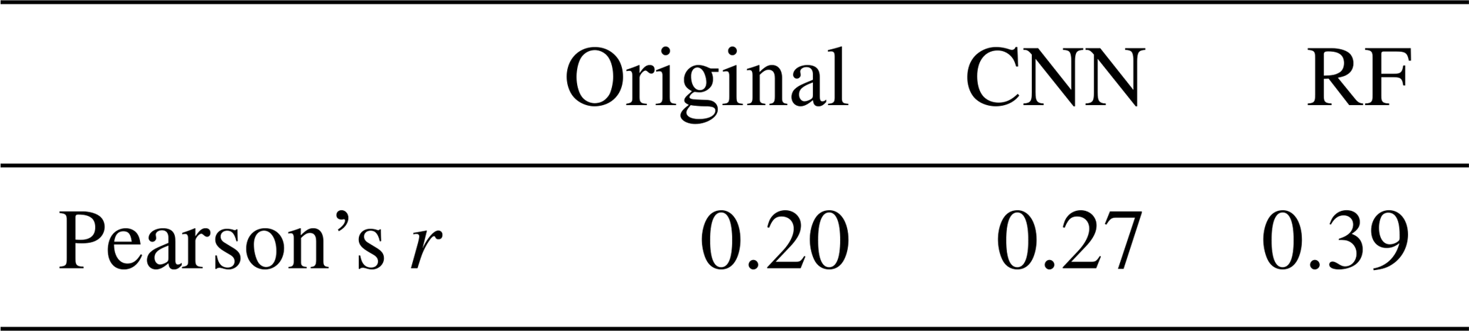
Our approach predicts TC for both topsoil and subsoil using a single model. The predictions benefit from using a common architecture for the two soil depths. When compared to predicting each depth separately using the random forest model, our method reduced the mean squared error by 15 % and 25 % for topsoil and subsoil, respectively. Other studies reported similar results to those produced by the random forest model. For example Kempen et al. (2011) reported an R² of 0.23 for the 30–60 cm depth range. Brus et al. (2016) also noticed a significant increase in the error for predicting organic carbon at deeper soil layers. Our results confirm the recent study of Padarian et al. (2019), who showed a substantial decrease in the error associated with the prediction of the deeper soil layer using the CNN. The authors showed that the CNN generates a representation of the vertical distribution of the soil profile, which reproduced closely the observed vertical distribution. Following Angelini et al. (2017) we also tested this by assessing the interrelation between topsoil and subsoil for the measured TC, for the TC predicted by the CNN or for the TC predicted using the RF model (Table 4). The CNN maintains the correlation between depths much better than the RF model, as shown by the value of the Pearson r correlation coefficient. This is an important finding which needs to be confirmed in further studies. Soil properties are often predicted depth by depth, which can result in predicting physically unrealistic soil profiles. In this study we showed that the deterministic behaviour of a depth function can be partly reproduced by the CNN.

We used three covariates to calibrate the CNN model. This might be a surprisingly small number compared to other studies on mapping with machine learning techniques (e.g. Nussbaum et al., 2018). However, this is a similar number compared to Padarian et al. (2019), who used four covariates for mapping organic carbon at a large scale. Further research will test the effect of the number of covariates on the CNN model calibration. We foresee a large increase in the computational load when using more covariates. This is because, in most studies on deep learning, only three colour channels are used. In this study we showed that only a small number of covariates was sufficient to provide satisfactory prediction accuracy.

Table 4Pearson's r correlation coefficient between the topsoil and subsoil TC for the original measurements of the test set, the predicted TC by the CNN and the predicted TC by the RF model.

Download Print Version | Download XLSX

Adapting the CNN for soil mapping poses some practical problems. We mention two of them along with our solution for future research.

Input images containing missing values are disregarded by the CNN during calibration and prediction. This means that (i) sampling locations close to the border of the area will be discarded from the analysis because their corresponding covariate images contain missing values and (ii) prediction will suffer from an edge effect; i.e. pixels at the edge of the area will not be predicted. This is a common problem when using a moving window operation in GIS. In our study, we padded the rows and columns of the covariates with −1, so as to avoid providing missing values to the model. The CNN is capable of predicting TC while learning that values containing −1 are missing values so that the subsequent prediction does not acknowledge an edge effect. We note that padding a value of −1 is an arbitrary choice which might not be right in another case study.
A CNN model takes more time to train and predict than a RF one. In our case study, it took 5 s to fit the RF model and about 30 s to predict about 600 000 centre of grid cells, using a standard four-core laptop. The CNN took 15 min to fit and 30 s to predict but requires preparing a 4-D matrix of size $n \times c \times w \times h$ for the training (n is the number of sampling locations) and for predicting (n is the number of prediction locations). This is tractable when the study area is small or for predicting on a coarse grid but becomes quickly computationally cumbersome for large-scale or high-resolution mapping. This is a new problem arising from using multiple covariates when image recognition problems commonly use three channels (colour channels RGB). A straightforward solution is to increase the number of cores available. Most available software implementations of deep learning models already support the use of parallel computing solutions.

Finally, we note that, in spite of its predictive power, the CNN has the major disadvantage of being a “black box” machine learning model, where results provide little knowledge, if any, on soil processes. In fact, many authors have noted that machine learning models are difficult to interpret. Recent publications (e.g. Angelini et al., 2017) have take a step toward “conscious” digital soil mapping where cause–effect relationships are adjusted with pedological knowledge. Solutions to interpret the CNN or more common ANN models exist but they have been unexplored in digital soil mapping, for example automated sensitivity analysis (Tickle et al., 1998) which consists in keeping track of the error computed during back propagation to measure the degree to which each covariate contributes to the prediction error. The larger the contribution, the larger the influence of the covariate. Another solution is to extract set of rules (Andrews et al., 1995) for each hidden layer based on the connection weight vector and associated bias of each neuron. Taking these methods into account would certainly make a valuable extension to future CNN studies.

6 Conclusions

We have shown how to train a deep learning model to predict total organic carbon at two soil depths using uncertain measurement of the soil property. The results and discussion bring us to the following conclusions.

The uncertainty of the organic carbon values inferred by NIR spectroscopy was larger than those inferred by MIR. The uncertainty of the NIR-inferred soil carbon measurement was large. Ignoring the latter uncertainty during model calibration results in a substantial part of the uncertainty being ignored, which can potentially lead to biased parameter estimates.
A known measurement error can easily be accounted for when calibrating a CNN model, by weighting the objective function to be optimized.
The CNN can be used for soil mapping using contextual covariate information. However the amount of contextual information we supply to the model, as represented by the window size of the input covariates, must be chosen with attention. In our case study a radius of 262 to 360 m provided the best results. This is closely related to the range of the soil organic carbon spatial autocorrelation. Future studies may show whether this is a consistent finding or case-dependent.
In our case study, the CNN outperforms the RF model as assessed by several prediction accuracy measures.
A single CNN model can be used to predict multiple outputs. In our case study, we predicted simultaneously at two soil depths. Deeper depth was much better predicted by the CNN than the RF model. In addition, the reported predictions preserve the interrelation between depths. The CNN is more suited for predicting correlated outputs. This also needs to be further investigated so as to generate rules.
More research is needed to (i) identify solutions for fast CNN soil data (pre-)processing for large-scale or high-resolution soil mapping, (ii) develop methods to interpret CNN models and extract pedological knowledge from the neural network, and (iii) derive uncertainty bounds of the predictions made by the CNN.

Data availability

The point data used in this study are the property of the University of Sydney and are not publicly available. The data may be requested from Budiman Minasny at the University of Sydney.

Competing interests

The authors declare that they have no conflict of interest.

Acknowledgements

Alexandre M. J.-C. Wadoux received funding from the European Union's Seventh Framework Programme for research, technological development and demonstration under grant agreement no. 607000. We thank David Lopez-Paz, Facebook AI Research, for valuable comments.

Review statement

This paper was edited by Axel Don and reviewed by Tomislav Hengl and Thorsten Behrens.

References

Abadi, M., Barham, P., Chen, J., Chen, Z., Davis, A., Dean, J., Devin, M., Ghemawat, S., Irving, G., Isard, M., Kudlur, M., Levenberg, J., Monga, R., Moore, S., Murray, D. G., Steiner, B., Tucker, P., Vasudevan, V., Warden, P., Wicke, M., Yu, Y., and Zheng, X.: Tensorflow: a system for large-scale machine learning, in: 12th USENIX Symposium on Operating Systems Design and Implementation, Vol. 16, 265–283, 2016. a

Allaire, J. and Chollet, F.: keras: R Interface to “Keras”, available at: https://CRAN.R-project.org/package=keras (last access: 1 March 2019), R package version 2.2.0, 2018. a

Andrews, R., Diederich, J., and Tickle, A. B.: Survey and critique of techniques for extracting rules from trained artificial neural networks, Knowl.-Based Syst., 8, 373–389, 1995. a

Angelini, M. E., Heuvelink, G., and Kempen, B.: Multivariate mapping of soil with structural equation modelling, Eur. J. Soil Sci., 68, 575–591, 2017. a, b

Behrens, T., Schmidt, K., Zhu, A.-X., and Scholten, T.: The ConMap approach for terrain-based digital soil mapping, Eur. J. Soil Sci., 61, 133–143, 2010a. a

Behrens, T., Zhu, A.-X., Schmidt, K., and Scholten, T.: Multi-scale digital terrain analysis and feature selection for digital soil mapping, Geoderma, 155, 175–185, 2010b. a, b

Behrens, T., Schmidt, K., Ramirez-Lopez, L., Gallant, J., Zhu, A.-X., and Scholten, T.: Hyper-scale digital soil mapping and soil formation analysis, Geoderma, 213, 578–588, 2014. a, b, c, d

Behrens, T., Schmidt, K., MacMillan, R. A., and Viscarra Rossel, R. A.: Multi-scale digital soil mapping with deep learning, Sci. Rep.-UK, 8, 15244–15244, 2018. a, b

Brus, D. J., Yang, R.-M., and Zhang, G.-L.: Three-dimensional geostatistical modeling of soil organic carbon: A case study in the Qilian Mountains, China, Catena, 141, 46–55, 2016. a

Demattê, J. A. M., Fongaro, C. T., Rizzo, R., and Safanelli, J. L.: Geospatial Soil Sensing System (GEOS3): A powerful data mining procedure to retrieve soil spectral reflectance from satellite images, Remote Sens. Environ., 212, 161–175, 2018. a

Farr, T. G., Rosen, P. A., Caro, E., Crippen, R., Duren, R., Hensley, S., Kobrick, M., Paller, M., Rodriguez, E., Roth, L., Seal, D., Shaffer, S., Shimada, J., Umland, J., Werner, M., Oskin, M., Burbank, D., and Alsdorf, D.: The shuttle radar topography mission, Rev. Geophys., 45, RG2004, https://doi.org/10.1029/2005RG000183, 2007. a

Gallant, J. C. and Dowling, T. I.: A multiresolution index of valley bottom flatness for mapping depositional areas, Water Resour. Res., 39, 4.1–4.13, 2003. a

Geeves, G., Cresswell, H., Murphy, B., Gessler, P., Chartres, C., Little, I., and Bowman, G.: The physical, chemical and morphological properties of soils in the wheat-belt of southern New South wales and northern Victoria, Aust. Division of Soils Occasional Report, CSIRO, Australia, 1995. a

Goodfellow, I., Bengio, Y., Courville, A., and Bengio, Y.: Deep learning, Vol. 1, MIT press, Cambridge, 2016. a, b

Grimm, R., Behrens, T., Märker, M., and Elsenbeer, H.: Soil organic carbon concentrations and stocks on Barro Colorado Island-Digital soil mapping using Random Forests analysis, Geoderma, 146, 102–113, 2008. a

Grinand, C., Arrouays, D., Laroche, B., and Martin, M. P.: Extrapolating regional soil landscapes from an existing soil map: sampling intensity, validation procedures, and integration of spatial context, Geoderma, 143, 180–190, 2008. a

Hengl, T., Nussbaum, M., Wright, M. N., Heuvelink, G. B., and Gräler, B.: Random forest as a generic framework for predictive modeling of spatial and spatio-temporal variables, PeerJ, 6, e5518, https://doi.org/10.7717/peerj.5518, 2018. a, b

Jian-Bing, W., Du-Ning, X., Xing-Yi, Z., Xiu-Zhen, L., and Xiao-Yu, L.: Spatial variability of soil organic carbon in relation to environmental factors of a typical small watershed in the black soil region, northeast China, Environ. Monit. Assess., 121, 597–613, 2006. a

Kempen, B., Brus, D., and Stoorvogel, J.: Three-dimensional mapping of soil organic matter content using soil type–specific depth functions, Geoderma, 162, 107–123, 2011. a

Kingma, D. P. and Ba, J.: Adam: A method for stochastic optimization, conference paper, 3rd International Conference for Learning Representations, San Diego, 2015. a

Kumhálová, J., Kumhála, F., Kroulík, M., and Matějková, Š.: The impact of topography on soil properties and yield and the effects of weather conditions, Precis. Agric., 12, 813–830, 2011. a

Lark, R. and Webster, R.: Changes in variance and correlation of soil properties with scale and location: analysis using an adapted maximal overlap discrete wavelet transform, Eur. J. Soil Sci., 52, 547–562, 2001. a

Lawrence, I. and Lin, K.: A concordance correlation coefficient to evaluate reproducibility, Biometrics, 45, 255–268, 1989. a

LeCun, Y., Boser, B., Denker, J. S., Henderson, D., Howard, R. E., Hubbard, W., and Jackel, L. D.: Backpropagation applied to handwritten zip code recognition, Neural Comput., 1, 541–551, 1989. a

LeCun, Y., Bengio, Y., and Hinton, G.: Deep learning, Nature, 521, 436–444, 2015. a

McBratney, A. B., Minasny, B., and Stockmann, U.: Pedometrics, Springer International Publishing, 2018. a

Miller, B. A., Koszinski, S., Wehrhan, M., and Sommer, M.: Impact of multi-scale predictor selection for modeling soil properties, Geoderma, 239, 97–106, 2015. a, b

Minasny, B., McBratney, A. B., and Salvador-Blanes, S.: Quantitative models for pedogenesis – A review, Geoderma, 144, 140–157, 2008. a

Moore, I. D., Gessler, P., Nielsen, G., and Peterson, G.: Soil attribute prediction using terrain analysis, Soil Sci. Soc. Am. J., 57, 443–452, 1993. a

Moran, C. J. and Bui, E. N.: Spatial data mining for enhanced soil map modelling, Int. J. Geogr. Inf. Sci., 16, 533–549, 2002. a

Nussbaum, M., Spiess, K., Baltensweiler, A., Grob, U., Keller, A., Greiner, L., Schaepman, M. E., and Papritz, A.: Evaluation of digital soil mapping approaches with large sets of environmental covariates, Soil, 4, 1–22, 2018. a, b

Padarian, J., Minasny, B., and McBratney, A. B.: Using deep learning for digital soil mapping, SOIL, 5, 79–89, https://doi.org/10.5194/soil-5-79-2019, 2019. a, b, c, d, e

Ramirez-Lopez, L., Wadoux, A. M. J.-C., Franceschini, M., Terra, F., Marques, K., Sayao, V. M., and Demattê, J.: Robust soil mapping at farm scale with vis-NIR spectroscopy, Eur. J. Soil Sci., in press, 2019. a, b, c

R Core Team: R: A Language and Environment for Statistical Computing, R Foundation for Statistical Computing, Vienna, Austria, available at: https://www.R-project.org/ (last access: 1 March 2019), 2018. a

Rossel, R. V., Walvoort, D., McBratney, A., Janik, L. J., and Skjemstad, J.: Visible, near infrared, mid infrared or combined diffuse reflectance spectroscopy for simultaneous assessment of various soil properties, Geoderma, 131, 59–75, 2006. a

Samuel-Rosa, A., Heuvelink, G., Vasques, G., and Anjos, L.: Do more detailed environmental covariates deliver more accurate soil maps?, Geoderma, 243, 214–227, 2015. a

Smith, M. P., Zhu, A.-X., Burt, J. E., and Stiles, C.: The effects of DEM resolution and neighborhood size on digital soil survey, Geoderma, 137, 58–69, 2006. a, b

Snoek, J., Larochelle, H., and Adams, R. P.: Practical bayesian optimization of machine learning algorithms, in: Advances in neural information processing systems, Curran Associates, Inc., New York, 2951–2959, 2012. a

Somarathna, P., Minasny, B., Malone, B. P., Stockmann, U., and McBratney, A. B.: Accounting for the measurement error of spectroscopically inferred soil carbon data for improved precision of spatial predictions, Sci. Total Environ., 631, 377–389, 2018. a, b, c

Tickle, A. B., Andrews, R., Golea, M., and Diederich, J.: The truth will come to light: Directions and challenges in extracting the knowledge embedded within trained artificial neural networks, IEEE T. Neural Networ., 9, 1057–1068, 1998. a

Wadoux, A. M. J.-C., Brus, D. J., and Heuvelink, G. B.: Accounting for non-stationary variance in geostatistical mapping of soil properties, Geoderma, 324, 138–147, 2018. a